Utilize Conditional Formatting with Formulas

Microsoft Excel’s conditional formatting with formulas is a powerful feature that allows users to visually enhance their data based on specific criteria.

Rather than manually scanning through rows and columns of numbers to find outliers or important trends, individuals can set up rules that automatically apply different formatting styles—like font colour, cell background, or border style—whenever cells meet certain conditions. This dynamic tool helps in making data analysis more efficient and in communicating key information at a glance.

Using formulas within conditional formatting, Excel users can go beyond the default rules based on cell values and create customised conditions. For example, they may highlight all cells that are above an average value or emphasise weekends and holidays in a date list.

Conditional formatting rules with formulas can reference other cells, perform calculations, and even utilise logical operators to create complex and robust data visualisations. This versatility opens up endless possibilities for data presentation, turning a simple spreadsheet into a clear and informative dashboard.

Creating these custom rules may seem daunting at first, but with a basic understanding of Excel formulas and some guidance, even beginners can start to apply conditional formatting with confidence.

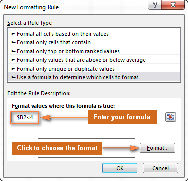
The formulas entered as part of these rules need to return a TRUE or FALSE value, which Excel uses to determine whether the formatting should be applied to the cell in question. With a bit of practice, this feature can significantly enhance the functionality and appearance of Excel spreadsheets.

---

Leveraging Formulas for Dynamic Formatting

Excel’s conditional formatting feature is significantly enhanced when combined with formulas, offering a dynamic approach to visualising data changes and criteria.

Understanding Conditional Formatting

Conditional formatting in Excel is a tool that alters the appearance of cells based on specific criteria. It allows for immediate visual cues about data, such as highlighting outliers or indicating trends. When one utilises formulas within conditional formatting, one opens a door to customisation, far beyond the standard preset options.

Using Formulas In Conditional Formatting

Applying formulas to conditional formatting involves crafting logical statements that return TRUE or FALSE. For instance, one might utilise the ISODD function to colour all odd rows for better readability. The process begins by selecting a range of cells, then choosing a formula that dictates the formatting—such as changing the background colour if a cell’s value exceeds a particular threshold.

Excel provides a platform for intricate formatting rules that respond to data dynamically. For example, if one wished to format cells based on another cell, a formula can reference other cells to determine the format. This interactivity allows for live updates as the data evolves, making one’s spreadsheets both functional and visually compelling.

Here’s more on this highly useful Excel functionality: