Often you’ll want to search a list of data – a list of toy products with prices in two columns for example – for a word (a particular product, say), to return a corresponding piece of data (the price of the product in our example).
So, using our simple example, we’d want our lookup function to search the following price list’s first column (for Lego Set, say) and then return the toy’s price ($52).

You may be already family with the VLOOKUP Excel function which does this quite well for such simple examples. However it struggles with more complex lookups.
For example suppose our toy store had branches in 3 different cities, all with different prices:

In order to obtain a toy price (a Doll in LA, say) we’d need to look up both the row, to find ‘Doll’, and the ‘LA’ column.
For these more complicated lookups we need two Excel functions:
- INDEX : Returns the value in table given its row and column numbers
- MATCH: searches rows and columns and returns the row and column numbers to be used in the INDEX look up
Below is a detailed explanation of how these two functions work:
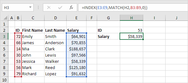
INDEX and MATCH
Use INDEX and MATCH in Excel and impress your boss. Instead of using VLOOKUP, use INDEX and MATCH. To perform advanced lookups, you’ll need INDEX and MATCH.